This page was generated from docs/Examples/LiquidusTests/LiquidusTest.ipynb. Interactive online version: .

Python Notebook Download

Using MELTS to find the liquidus temperature

• Finding the liquidus temperature of a magma is one of the first steps of most crystallisation and/or decompression calculations.

• Usually this command is used as part of the isobaric_crystallisation and isothermal_decompression functions (amongst others).

• However, it’s still useful to consider how the liquidus function works independently, and examine how well MELTS performs as a Thermometer in igneous systems.

Before any calculations can be run users need to download and install the alphaMELTS for Python files. This can be easily achieved with one simple function, please see the installation guide available on ReadTheDocs.

Data used in the calculations below can be downloaded from here: https://github.com/gleesonm1/PetThermoTools/blob/master/docs/Examples/LiquidusTests/MELTS_MAGEMin_Liquidus.xlsx

import numpy as np
import pandas as pd
import matplotlib.pyplot as plt
import petthermotools as ptt
from tqdm.notebook import tqdm, trange
# import pickle

# If the alphaMELTS for Python files have not been added to your Python path (see installation guide) then use the two lines below to add
# the location of the alphaMELTS files here.
# import sys
# sys.path.append(r'path_to_alphaMELTS_files')

alphaMELTS for Python files successfully located.
If using the Green et al. (2025) or Weller et al. (2024) thermodynamic models please run `ptt.activate_petthermotools_env()` prior to any calculations.

import platform
if platform.system() == "Darwin":
    # used to suppress MELTS outputs in MacOS systems (run twice)
    import sys
    import os
    sys.stdout = open(os.devnull, 'w')
    sys.stderr = open(os.devnull, 'w')

To test the ability of MELTS to act as a liquid-only thermometer we need some experiments to test them against. Here, we use a database of experimental data compiled by P. Wieser (Wieser et al. 2025).

Data = pd.read_excel('MELTS_MAGEMIN_Liquidus.xlsx')
Data = Data[~np.isinf(Data["H2O_Liq"])]
Data = Data.reset_index(drop=True)

The entire experimental dataset contains over 2000 samples. Therefore, to reduce the computational time in this example I isolate 200 experiments (randomly selected) to be used in the following calculations. A new DataFrame is constructed using only these experiments.

# randomly select 200 rows from the original DataFrame
Ch = np.random.choice(range(len(Data['SiO2_Liq'])), 200, replace=False)
Test = Data.copy()
Test = Test.loc[Ch]

# reset the index in the new DataFrame
Test = Test.reset_index(drop = True)
Test = Test.dropna()

Now that we have this ‘Test’ DataFrame we can use the findLiq_multi function to identify the liquidus temperature of each sample. Ideally, we’d have information about either the Fe redox state or an estimate of the oxygen fugacity of each melt. Unfortunately, we don’t have this information for every sample so instead we will define a constant Fe\(^{3+}\)/Fe\(_{tot}\) ratio for all samples:

Results_pMELTS = ptt.findLiq_multi(Model = "pMELTS", # which MELTS model to use - "pMELTS", "MELTSv1.0.2", "MELTSv1.1.0", or "MELTSv1.2.0"
                        bulk = Test, # initial composition(s) wither a dictionary (if one composition) or a DataFrame (multiple compositions)
                        P_bar = Test['P_kbar'].values*1000, # Pressure (in bars) of the calculation
                        Fe3Fet_Liq = 0.15) # initial Fe3Fet_Liq ratio of the sample(s)

Examining the results reveals the information that is recorded by this function. Notably, the findLiq_multi code will return the composition of the melt at the liquidus (in wt% hydrous normalized), whether or not the melt is fluid saturated at the liquidus, the liquidus phase, and (critically) the liquidus temperature (in degrees Celsius).

Results_pMELTS.head()

	T_Liq_C	liquidus_phase	fluid_saturated	SiO2_Liq	TiO2_Liq	Al2O3_Liq	Cr2O3_Liq	FeOt_Liq	MnO_Liq	MgO_Liq	CaO_Liq	Na2O_Liq	K2O_Liq	P2O5_Liq	H2O_Liq	CO2_Liq	Fe3Fet_Liq
0	885.045528	alkali-feldspar1	No	72.391194	0.210721	12.905554	0.000000	1.388716	0.143674	0.229878	1.331236	2.920335	4.143710	0.000000	4.334981	0.0	0.149921
1	1072.731916	clinopyroxene1	No	64.247513	0.503895	15.601725	0.000000	3.369638	0.087215	2.112275	4.864294	4.418883	1.376060	0.155049	3.263454	0.0	0.149919
2	1173.805892	clinopyroxene1	No	49.242231	1.054271	17.036641	0.000000	6.408268	0.141980	4.024817	8.881612	2.261485	0.557779	0.273819	10.117096	0.0	0.149904
3	978.379922	plagioclase1	No	61.273117	0.165254	17.596388	0.092955	4.048346	0.000000	2.344540	5.782476	3.191111	0.123935	0.206567	5.175310	0.0	0.149921
4	1067.517453	plagioclase1	No	60.388184	1.634061	15.426604	0.000000	6.474746	0.243587	2.293775	6.038702	3.765357	1.603601	0.304483	1.826900	0.0	0.149921

In this initial calculation, the liquidus temperature is calculated using the pMELTS model, which was designed for use on mantle-like bulk compositions at 1 - 3 GPa (Ghiorso et al. 2002). For the majorty of samples in this database it may be more appropriate to use the rhyoliteMELTSv1.0.2 (Gualda et al. 2012) or rhyoliteMELTSv1.2.0 (Ghiorso and Gualda, 2015) models. We can rerun the same calculations but change the Model selected:

Results_MELTSv102 = ptt.findLiq_multi(Model = "MELTSv1.0.2", # which MELTS model to use - "pMELTS", "MELTSv1.0.2", "MELTSv1.1.0", or "MELTSv1.2.0"
                        bulk = Test, # initial composition(s) wither a dictionary (if one composition) or a DataFrame (multiple compositions)
                        P_bar = Test['P_kbar'].values*1000, # Pressure (in bars) of the calculation
                        Fe3Fet_Liq = 0.15) # initial Fe3Fet_Liq ratio of the sample(s)

Results_MELTSv102.head()

	T_Liq_C	liquidus_phase	fluid_saturated	SiO2_Liq	TiO2_Liq	Al2O3_Liq	Cr2O3_Liq	FeOt_Liq	MnO_Liq	MgO_Liq	CaO_Liq	Na2O_Liq	K2O_Liq	P2O5_Liq	H2O_Liq	CO2_Liq	Fe3Fet_Liq
0	812.145528	orthopyroxene1	No	72.389212	0.210658	12.907554	0.000000	1.388024	0.143630	0.229674	1.330969	2.920481	4.146126	0.000000	4.333671	0.0	0.149947
1	1112.431916	orthopyroxene1	No	64.247577	0.503913	15.601925	0.000000	3.369405	0.087216	2.111717	4.864680	4.418948	1.376076	0.155051	3.263493	0.0	0.149932
2	1251.505892	garnet1	Yes	50.284931	1.077134	17.394800	0.000000	6.542481	0.144999	4.108213	9.071375	2.309623	0.569638	0.279640	8.217166	0.0	0.149980
3	1031.379922	spinel1	No	61.272114	0.165237	17.597781	0.092926	4.047913	0.000000	2.344301	5.783311	3.191148	0.123928	0.206547	5.174793	0.0	0.149919
4	1063.117453	orthopyroxene1	No	60.388161	1.634050	15.427047	0.000000	6.474469	0.243585	2.293422	6.038864	3.765425	1.603604	0.304482	1.826891	0.0	0.149925

Results_MELTSv120 = ptt.findLiq_multi(Model = "MELTSv1.2.0", # which MELTS model to use - "pMELTS", "MELTSv1.0.2", "MELTSv1.1.0", or "MELTSv1.2.0"
                        bulk = Test, # initial composition(s) wither a dictionary (if one composition) or a DataFrame (multiple compositions)
                        P_bar = Test['P_kbar'].values*1000, # Pressure (in bars) of the calculation
                        Fe3Fet_Liq = 0.15) # initial Fe3Fet_Liq ratio of the sample(s)

Results_MELTSv120.head()

	T_Liq_C	liquidus_phase	fluid_saturated	SiO2_Liq	TiO2_Liq	Al2O3_Liq	Cr2O3_Liq	FeOt_Liq	MnO_Liq	MgO_Liq	CaO_Liq	Na2O_Liq	K2O_Liq	P2O5_Liq	H2O_Liq	CO2_Liq	Fe3Fet_Liq
0	849.145528	plagioclase1	No	72.390605	0.210686	12.905835	0.000000	1.388483	0.143649	0.229839	1.330329	2.919742	4.146581	0.000000	4.334251	0.0	0.149921
1	1082.531916	orthopyroxene1	No	64.247730	0.503916	15.602032	0.000000	3.369230	0.087217	2.111482	4.864723	4.418996	1.376092	0.155053	3.263529	0.0	0.149937
2	1234.505892	garnet1	No	49.242979	1.054757	17.034953	0.000000	6.407019	0.141987	4.024033	8.883451	2.261643	0.557804	0.273831	10.117545	0.0	0.149969
3	1100.279922	spinel1	No	61.272250	0.165237	17.597781	0.092859	4.047827	0.000000	2.344288	5.783323	3.191155	0.123928	0.206547	5.174805	0.0	0.149911
4	1065.217453	plagioclase1	No	60.388328	1.634091	15.426328	0.000000	6.474865	0.243591	2.293817	6.038577	3.765345	1.603633	0.304489	1.826934	0.0	0.149921

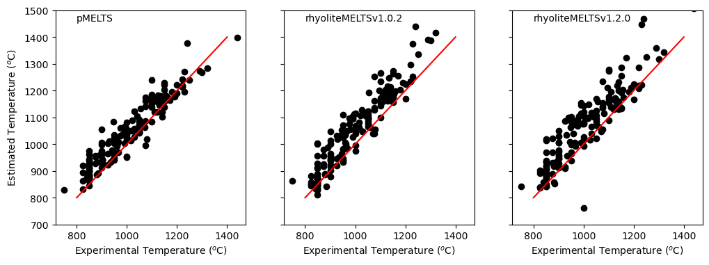
Now that we have the results of this analysis, we can compare the results of these calculations to the true experimental temperature. Experiments that have no reported water typically show a very poor match to the experimental temperature, and are thus excluded from the following comparison. Additionally, we exlude any calculations that did not return a result (Results[‘T_C_liq’] = 0).

Overall, MELTS does an acceptable job in reproducing the experimental temperatures, although it is notable that the liquidus temperature is typically overpredicted by around 50 \(^{o}\)C.

f, a = plt.subplots(1,3, figsize = (12,4), sharex = True, sharey = True)

a[0].plot(Test['T_K'][(Test['H2O_Liq'] > 0) & (Results_pMELTS['T_Liq_C'] > 0)]-273.15,
       Results_pMELTS['T_Liq_C'][(Test['H2O_Liq'] > 0) & (Results_pMELTS['T_Liq_C'] > 0)],
        'ok')
a[0].plot([800,1400],[800,1400], 'r-')
a[0].set_ylabel('Estimated Temperature ($^{o}$C)')
a[0].set_xlabel('Experimental Temperature ($^{o}$C)')
a[0].text(800, 1460, 'pMELTS')


a[1].plot(Test['T_K'][(Test['H2O_Liq'] > 0) & (Results_MELTSv102['T_Liq_C'] > 0)]-273.15,
       Results_MELTSv102['T_Liq_C'][(Test['H2O_Liq'] > 0) & (Results_MELTSv102['T_Liq_C'] > 0)],
        'ok')
a[1].plot([800,1400],[800,1400], 'r-')
a[1].set_xlabel('Experimental Temperature ($^{o}$C)')
a[1].text(800, 1460, 'rhyoliteMELTSv1.0.2')


a[2].plot(Test['T_K'][(Test['H2O_Liq'] > 0) & (Results_MELTSv120['T_Liq_C'] > 0)]-273.15,
       Results_MELTSv120['T_Liq_C'][(Test['H2O_Liq'] > 0) & (Results_MELTSv120['T_Liq_C'] > 0)],
        'ok')
a[2].plot([800,1400],[800,1400], 'r-')
a[2].set_xlabel('Experimental Temperature ($^{o}$C)')
a[2].text(800, 1460, 'rhyoliteMELTSv1.2.0')

a[2].set_ylim([700,1500])

(700.0, 1500.0)