This page was generated from
docs/Examples/CrystallisationTests/BasalticCrystallisation_withMAGEMin.ipynb.
Interactive online version:
![]() .
.
Modelling liquid-line-of-descents with MAGEMin
One of the primary uses of the MELTS models is simulating the crystallisation of magma under different conditions.
Useful for identifying whether samples are linked by crystallisation or if other processes are required to explain the geochemical variability of a region.
While crystallization models have traditionally been run using the MELTs thermodynamic models to development of MAGEMin allows us to simulate fractional crystallization using alternative thermodynamic models (Green et al. 2025; Weller et al. 2024).
Before any calculations can be run users need to make sure they have followed the instructions for installing juliacall and the necessary MAGEMin packages in the installation guide.
Data used in the calculations below can be downloaded from here: https://github.com/gleesonm1/PetThermoTools/blob/master/docs/Examples/CrystallisationTests/Fernandina_glass.xlsx
[1]:
import numpy as np
import pandas as pd
import matplotlib.pyplot as plt
import petthermotools as ptt

import os

# os.environ["JULIA_PROJECT"] = os.path.expanduser("~/.petthermotools_julia_env")
# os.environ["PYTHON_JULIACALL_AUTOLOAD_IPYTHON_EXTENSION"] = "no"

ptt.activate_petthermotools_env()
alphaMELTS for Python files successfully located.
If using the Green et al. (2025) or Weller et al. (2024) thermodynamic models please run `ptt.activate_petthermotools_env()` prior to any calculations.
Julia environment detected.
Detected IPython. Loading juliacall extension. See https://juliapy.github.io/PythonCall.jl/stable/compat/#IPython
  Activating project at `~/.petthermotools_julia_env`
Precompiling MAGEMinCalc...
    780.0 ms  ? PythonCall
Info Given MAGEMinCalc was explicitly requested, output will be shown live
Using libMAGEMin.dylib from MAGEMin_jll
┌ Warning: Module PythonCall with build ID fafbfcfd-5919-c725-0476-cd0238baa5be is missing from the cache.
│ This may mean PythonCall [6099a3de-0909-46bc-b1f4-468b9a2dfc0d] does not support precompilation but is imported by a module that does.
└ @ Base loading.jl:2541
   1196.0 ms  ? MAGEMinCalc
[ Info: Precompiling MAGEMinCalc [dd69d18c-a947-4316-a873-d8ea006ff1b2] (cache misses: wrong dep version loaded (4), mismatched flags (2))
Using libMAGEMin.dylib from MAGEMin_jll
Using libMAGEMin.dylib from MAGEMin_jll
      From worker 5:    Using libMAGEMin.dylib from MAGEMin_jll
      From worker 3:    Using libMAGEMin.dylib from MAGEMin_jll
      From worker 2:    Using libMAGEMin.dylib from MAGEMin_jll
      From worker 4:    Using libMAGEMin.dylib from MAGEMin_jll
Julia Environment Ready. MAGEMinCalc v0.6.1 detected
┌ Warning: Module PythonCall with build ID fafbfcfd-5919-c725-0476-cd0238baa5be is missing from the cache.
│ This may mean PythonCall [6099a3de-0909-46bc-b1f4-468b9a2dfc0d] does not support precompilation but is imported by a module that does.
└ @ Base loading.jl:2541
┌ Info: Skipping precompilation due to precompilable error. Importing MAGEMinCalc [dd69d18c-a947-4316-a873-d8ea006ff1b2].
└   exception = Error when precompiling module, potentially caused by a __precompile__(false) declaration in the module.
In this notebook we’ll show how PetThermoTools can quickly perform multiple calculations (utilizing parallel processing), and investigate how the liquid-line-of-descent is linked to the conditions of magma storage. Note: this notebook is near identical to the standard liquid-line-of-descent example but uses the Green et al. (2025) and Weller et al. (2024) thermodynamic models through MAGEMin; Riel et al. (2022).
First, we need to load in some data. For this example we’ll use data from Isla Fernandina in the Galapagos Archipelago, where a series of melt inclusions (Koleszar et al. 2009) and matrix glasses (Peterson et al. 2017) provide us with plenty of glass data to constain the magmatic evolution of the sub-volcanic system. The melt inclusion and matrix glass data is included in a single excel spreadsheet that we can load in using Pandas. We can also split this DataFrame into two. One containing just the melt inclusion data, the second including just the matrix glass data.
[2]:
df = pd.read_excel('Fernandina_glass.xlsx')
df = df.fillna(0)

# split data based on the Group (Melt Inclusion or Matrix Glass)
MI = df.loc[df['Group'] == 'MI',:].reset_index(drop = True)
MG = df.loc[df['Group'] == 'MG',:].reset_index(drop = True)

MG.head()
[2]:
| Group | Latitude | Longitude | SiO2 | TiO2 | Al2O3 | FeOt | MnO | MgO | CaO | Na2O | K2O | P2O5 | H2O | CO2 | |
|---|---|---|---|---|---|---|---|---|---|---|---|---|---|---|---|
| 0 | MG | -0.17 | -91.77 | 49.11 | 2.90 | 14.04 | 11.38 | 0.21 | 6.53 | 11.88 | 2.55 | 0.43 | 0.30 | 0.593 | 0.011442 |
| 1 | MG | -0.17 | -91.77 | 49.22 | 3.10 | 14.09 | 11.37 | 0.20 | 6.75 | 11.78 | 2.75 | 0.44 | 0.31 | 0.683 | 0.009890 |
| 2 | MG | -0.21 | -91.81 | 49.01 | 2.92 | 13.92 | 11.74 | 0.21 | 6.31 | 11.90 | 2.55 | 0.46 | 0.33 | 0.635 | 0.012210 |
| 3 | MG | -0.21 | -91.80 | 49.42 | 3.14 | 13.92 | 11.77 | 0.20 | 6.47 | 11.46 | 2.82 | 0.46 | 0.33 | 0.732 | 0.010531 |
| 4 | MG | -0.24 | -91.75 | 48.76 | 3.57 | 13.88 | 11.83 | 0.23 | 6.37 | 11.40 | 3.09 | 0.52 | 0.36 | 0.834 | 0.007797 |
One of the key things that we need to perform any calculations with MELTS is a starting composition. To start, let’s use the most primitive (highest MgO) composition from the melt inclusion analyses. There are a few ways to find this composition, the way I like to do so (not necessarily the quickest) is to simply sort the melt inclusion DataFrame by the MgO contents and select the first row:
[3]:
MI = MI.sort_values('MgO', ascending = False, ignore_index = True)
MI.head()
[3]:
| Group | Latitude | Longitude | SiO2 | TiO2 | Al2O3 | FeOt | MnO | MgO | CaO | Na2O | K2O | P2O5 | H2O | CO2 | |
|---|---|---|---|---|---|---|---|---|---|---|---|---|---|---|---|
| 0 | MI | 0.0 | 0.0 | 47.5 | 2.29 | 16.4 | 9.16 | 0.123 | 9.38 | 11.6 | 2.25 | 0.329 | 0.257 | 0.68 | 0.0280 |
| 1 | MI | 0.0 | 0.0 | 47.5 | 2.58 | 15.5 | 10.04 | 0.138 | 8.97 | 11.4 | 2.44 | 0.428 | 0.262 | 0.69 | 0.0630 |
| 2 | MI | 0.0 | 0.0 | 49.2 | 2.33 | 16.0 | 8.67 | 0.147 | 8.94 | 12.0 | 1.78 | 0.005 | 0.094 | 0.78 | 0.0004 |
| 3 | MI | 0.0 | 0.0 | 48.4 | 2.50 | 15.7 | 9.07 | 0.139 | 8.88 | 11.6 | 2.18 | 0.398 | 0.326 | 0.69 | 0.0126 |
| 4 | MI | 0.0 | 0.0 | 48.1 | 2.46 | 15.3 | 8.96 | 0.153 | 8.82 | 12.1 | 2.34 | 0.325 | 0.387 | 0.88 | 0.4986 |
[4]:
starting_comp = MI.loc[0]
starting_comp['Cr2O3'] = 0.05
starting_comp
[4]:
Group           MI
Latitude       0.0
Longitude      0.0
SiO2          47.5
TiO2          2.29
Al2O3         16.4
FeOt          9.16
MnO          0.123
MgO           9.38
CaO           11.6
Na2O          2.25
K2O          0.329
P2O5         0.257
H2O           0.68
CO2          0.028
Cr2O3         0.05
Name: 0, dtype: object
We can now perform crystallisation calculations. These calculations are run using the Weller et al. (2024) thermodynamic model, start at the liquidus and end at 1100\(^o\)C. The calculations are also run at 1 log unit below the FMQ buffer. By specifying Frac_solid = True, we inform PetThermoTools that we want to perform a fractional (rather than equilibrium) crystallisation scenario.
[5]:
Weller_Xtal = ptt.isobaric_crystallisation(Model = "Weller2024",
                                           bulk = starting_comp.to_dict(),
                                           find_liquidus = True,
                                           P_bar = np.array([500.0,1000.0,2000.0,4000.0]),
                                           T_end_C = 1100.0,
                                           dt_C = 2.0,
                                           fO2_buffer = "FMQ",
                                           fO2_offset = -1.0,
                                           label = 'P_bar',
                                           Frac_solid = True,
                                           timeout = 300)
We can also run the same calculations using the Green et al. (2025) thermodynamic model (through MAGEMin_C).
[6]:
Green_Xtal = ptt.isobaric_crystallisation(Model = "Green2025",
                                           bulk = starting_comp.to_dict(),
                                           find_liquidus = True,
                                           P_bar = np.array([500.0,1000.0,2000.0,4000.0]),
                                           T_end_C = 1100.0,
                                           dt_C = 2.0,
                                           fO2_buffer = "FMQ",
                                           fO2_offset = -1.0,
                                           label = 'P_bar',
                                           Frac_solid = True,
                                           timeout = 300)
There are several ways to display the results. Option 1 is to use the in-built harker plotting function which directly plots a 3-by-2 group of plots without having to make any changes to the output from the crystallisation models. You’ll see below that the code also allows other data to be loaded and plotted alongside the models:
[7]:
ptt.harker(Results = Weller_Xtal,  data = {'MI': MI, 'MG': MG},
    d_color = ['b','red'], legend_loc = [1,2])
y axis variable  Cr2O3 not found in data
y axis variable  Cr2O3 not found in data
[7]:
(<Figure size 960x900 with 9 Axes>,
 array([[<Axes: xlabel='MgO', ylabel='SiO$_2$'>,
         <Axes: xlabel='MgO', ylabel='TiO$_2$'>,
         <Axes: xlabel='MgO', ylabel='Al$_2$O$_3$'>],
        [<Axes: xlabel='MgO', ylabel='Cr$_2$O$_3$'>,
         <Axes: xlabel='MgO', ylabel='FeO$_t$'>,
         <Axes: xlabel='MgO', ylabel='CaO'>],
        [<Axes: xlabel='MgO', ylabel='Na$_2$O'>,
         <Axes: xlabel='MgO', ylabel='K$_2$O'>, <Axes: >]], dtype=object))
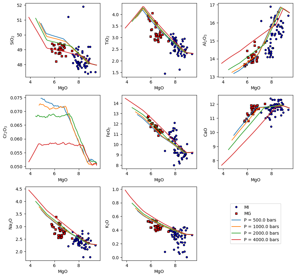
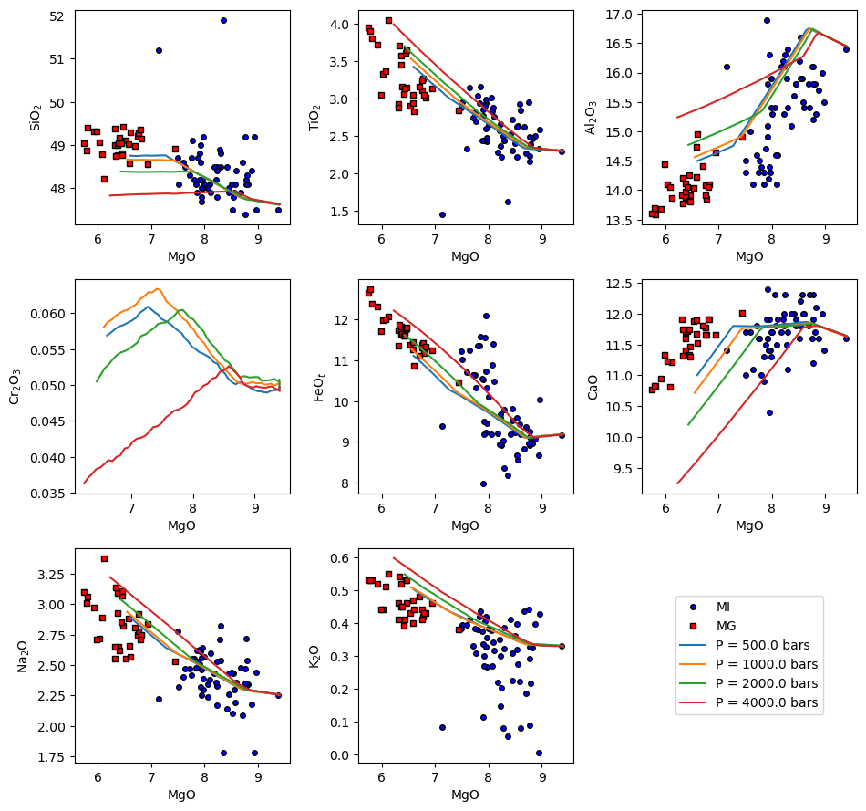
The plot above shows the results using the Weller et al. (2024) model. To plot the results of the Green et al. (2025) calculations we just need to change the parameter passed to the Results kwarg:
[8]:
ptt.harker(Results = Green_Xtal,  data = {'MI': MI, 'MG': MG},
    d_color = ['b','red'], legend_loc = [1,2])
y axis variable  Cr2O3 not found in data
y axis variable  Cr2O3 not found in data
[8]:
(<Figure size 960x900 with 9 Axes>,
 array([[<Axes: xlabel='MgO', ylabel='SiO$_2$'>,
         <Axes: xlabel='MgO', ylabel='TiO$_2$'>,
         <Axes: xlabel='MgO', ylabel='Al$_2$O$_3$'>],
        [<Axes: xlabel='MgO', ylabel='Cr$_2$O$_3$'>,
         <Axes: xlabel='MgO', ylabel='FeO$_t$'>,
         <Axes: xlabel='MgO', ylabel='CaO'>],
        [<Axes: xlabel='MgO', ylabel='Na$_2$O'>,
         <Axes: xlabel='MgO', ylabel='K$_2$O'>, <Axes: >]], dtype=object))
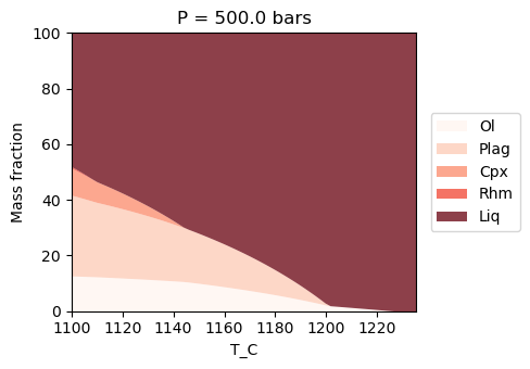
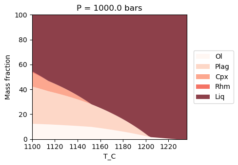
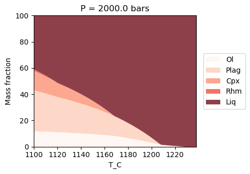
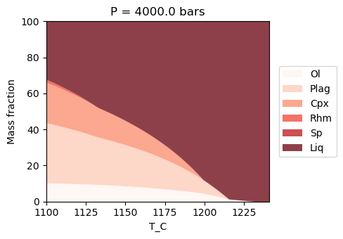
We can also examine the phase proportions estimated using the Weller et al. (2024) model:
[9]:
f, a = ptt.phase_plot(Weller_Xtal, x_axis = 'T_C',
                       cmap = "Reds")
[ ]:
[ ]: